Advanced Operations, Detecting Faces and Features

python

datacamp

machine learning

deep learning

neural network

Author

kakamana

Published

April 8, 2023

Advanced Operations, Detecting Faces and Features

As a result of completing this chapter, you will have a deeper understanding of image processing since you will be able to detect edges, corners, and even faces! Not only will you learn how to detect front faces, but also profile faces, cats, and dogs as well. Your skills will be applied to more complex real-world applications. With only a few lines of code, you will be able to master several widely used image processing techniques!

This Advanced Operations, Detecting Faces and Features is part of Datacamp course: Image Processing in Python There are images everywhere! Today, images contain a great deal of information that is sometimes difficult to access. Thus, image pre-processing has become a highly valuable skill, applicable to a wide range of applications. As a result of taking this course, you will be able to process, transform, and manipulate images at your discretion, no matter how many there are. Additionally, you will learn how to use scikit-image to restore damaged images, perform noise reduction, smart-resize images, count the number of dots on a dice, apply facial detection, and much more. You will be able to apply your knowledge of machine learning and artificial intelligence, machine and robotic vision, space and medical image analysis, retailing, and many other fields after completing this course. Take the step and dive into the wonderful world of computer vision!

This is my learning experience of data science through DataCamp. These repository contributions are part of my learning journey through my graduate program masters of applied data sciences (MADS) at University Of Michigan, DeepLearning.AI, Coursera & DataCamp. You can find my similar articles & more stories at my medium & LinkedIn profile. I am available at kaggle & github blogs & github repos. Thank you for your motivation, support & valuable feedback.

These include projects, coursework & notebook which I learned through my data science journey. They are created for reproducible & future reference purpose only. All source code, slides or screenshot are intellactual property of respective content authors. If you find these contents beneficial, kindly consider learning subscription from DeepLearning.AI Subscription, Coursera, DataCamp

Code

import numpy as np
import matplotlib.pyplot as plt
from skimage.io import imread

plt.rcParams['figure.figsize'] = (10, 8)

Finding the edges with Canny

Edges

In this exercise you will identify the shapes in a grapefruit image by detecting the edges, using the Canny algorithm.

Code

def show_image(image, title='Image', cmap_type='gray'):
    plt.imshow(image, cmap=cmap_type)
    plt.title(title)
    plt.axis('off')

def plot_comparison(img_original, img_filtered, img_title_filtered):
    fig, (ax1, ax2) = plt.subplots(ncols=2, figsize=(10, 8), sharex=True, sharey=True)
    ax1.imshow(img_original, cmap=plt.cm.gray)
    ax1.set_title('Original')
    ax1.axis('off')
    ax2.imshow(img_filtered, cmap=plt.cm.gray)
    ax2.set_title(img_title_filtered)
    ax2.axis('off')

Code

from skimage.feature import canny
from skimage import color

grapefruit = imread('dataset/toronjas.jpg')

# Convert image to grayscale
grapefruitb = color.rgb2gray(grapefruit)

# Apply canny edge detector
canny_edges = canny(grapefruitb)

# Show resulting image
plot_comparison(grapefruit, canny_edges, "Edges with Canny")
#show_image(grapefruit,"grapefruit")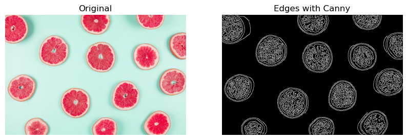

Less edgy

Let’s now try to spot just the outer shape of the grapefruits, the circles. You can do this by applying a more intense Gaussian filter to first make the image smoother. This can be achieved by specifying a bigger sigma in the canny function.

In this exercise, you’ll experiment with sigma values of the canny() function.

Code

edges_1_8 = canny(grapefruitb, sigma=1.8)

# Apply canny edge detector with a sigma of 2.2
edges_2_2 = canny(grapefruitb, sigma=2.2)

# Show resulting image
plot_comparison(edges_1_8, edges_2_2, 'change sigma from 1.8 to 2.2')

Right around the corner

Perspective

In this exercise, you will detect the corners of a building using the Harris corner detector.

Code

def show_image_with_corners(image, coords, title="Corners detected"):
    plt.imshow(image, interpolation='nearest', cmap='gray')
    plt.title(title)
    plt.plot(coords[:, 1], coords[:, 0], '+r', markersize=15)
    plt.axis('off')

Code

from skimage.feature import corner_harris, corner_peaks

building_image = imread('dataset/corners_building_top.jpg')

# Convert image from RGB to grayscale
building_image_gray = color.rgb2gray(building_image)

# Apply the detector to measure the possible corners
measure_image = corner_harris(building_image_gray)

# Find the peaks of the corners using the Harris detector
coords = corner_peaks(measure_image, min_distance=2)

# Show original and resulting image with corners detected
show_image(building_image, 'Original')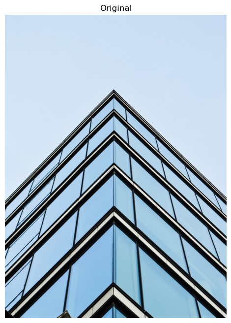

Code

show_image_with_corners(building_image, coords)

Less corners

In this exercise, you will test what happens when you set the minimum distance between corner peaks to be a higher number. Remember you do this with the min_distance attribute parameter of the corner_peaks() function.

Code

coords_w_min_2 = corner_peaks(measure_image, min_distance=2)
print("With a min_distance set to 2, we detect a total", len(coords_w_min_2), "corners in the image.")

# Find the peaks with a min distance of 40 pixels
coords_w_min_40 = corner_peaks(measure_image, min_distance=40)
print('With a min_distance set to 40, we detect a total', len(coords_w_min_40), 'corners in the image.')

With a min_distance set to 2, we detect a total 10696 corners in the image.
With a min_distance set to 40, we detect a total 58 corners in the image.

Code

show_image_with_corners(building_image, coords_w_min_2, "Corners detected with 2 px of min_distance")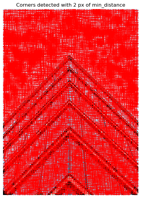

Code

show_image_with_corners(building_image, coords_w_min_40, "Corners detected with 40 px of min_distance")

Face detection

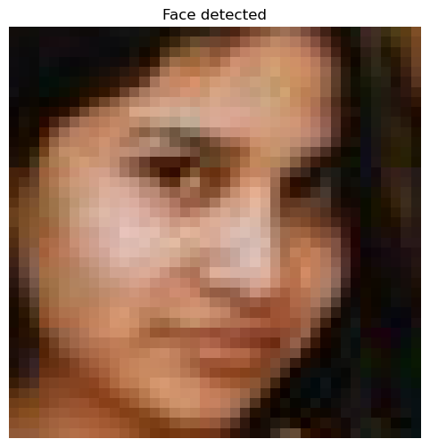
Is someone there? In this exercise, you will check whether or not there is a person present in an image taken at night.

Code

import matplotlib.patches as patches

def crop_face(result, detected, title="Face detected"):
    for d in detected:
        print(d)
        rostro= result[d['r']:d['r']+d['width'], d['c']:d['c']+d['height']]

        plt.figure(figsize=(8, 6))
        plt.imshow(rostro)
        plt.title(title)
        plt.axis('off')
        plt.show()

def show_detected_face(result, detected, title="Face image"):
    plt.figure()
    plt.imshow(result)
    img_desc = plt.gca()
    plt.set_cmap('gray')
    plt.title(title)
    plt.axis('off')

    for patch in detected:

        img_desc.add_patch(
            patches.Rectangle(
                (patch['c'], patch['r']),
                patch['width'],
                patch['height'],
                fill=False,
                color='r',
                linewidth=2)
        )
    plt.show()
    crop_face(result, detected)

Code

from skimage import data
from skimage.feature import Cascade

night_image = imread('dataset/face_det3.jpg')

# Load the trained file from data
trained_file = data.lbp_frontal_face_cascade_filename()

# Initialize the detector cascade
detector = Cascade(trained_file)

# Detect faces with min and max size of searching window
detected = detector.detect_multi_scale(img=night_image, scale_factor=1.2,
                                       step_ratio=1, min_size=(10, 10), max_size=(200, 200))

# Show the detected faces
show_detected_face(night_image, detected)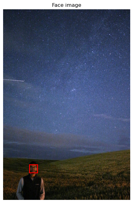

{'r': 774, 'c': 131, 'width': 40, 'height': 40}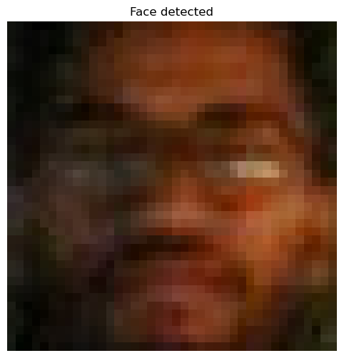

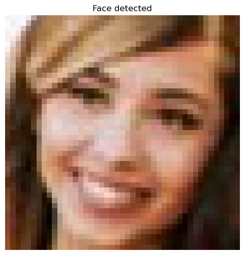
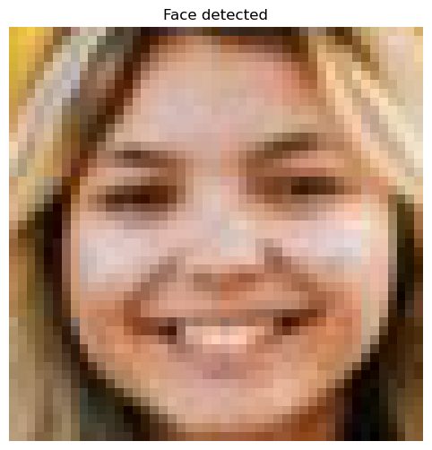
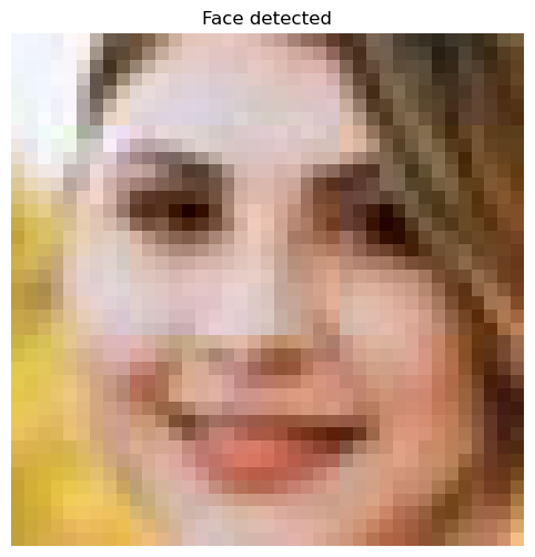
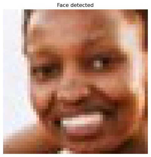
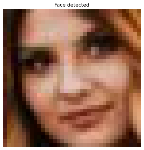
Multiple faces

In this exercise, you will detect multiple faces in an image and show them individually. Think of this as a way to create a dataset of your own friends’ faces!

Code

friends_image = imread('dataset/face_det_friends22.jpg')

# Detect faces with scale factor to 1.2 and step ratio to 1
detected = detector.detect_multi_scale(img=friends_image,
                                       scale_factor=1.2,
                                       step_ratio=1,
                                       min_size=(10, 10),
                                       max_size=(200, 200))

# Show detected faces
show_detected_face(friends_image, detected)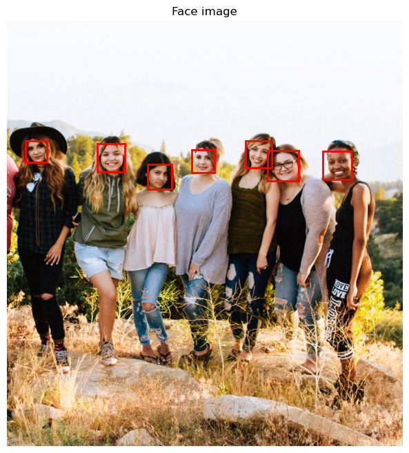

{'r': 218, 'c': 440, 'width': 52, 'height': 52}
{'r': 202, 'c': 402, 'width': 45, 'height': 45}
{'r': 207, 'c': 152, 'width': 47, 'height': 47}
{'r': 217, 'c': 311, 'width': 39, 'height': 39}
{'r': 219, 'c': 533, 'width': 48, 'height': 48}
{'r': 242, 'c': 237, 'width': 41, 'height': 41}
{'r': 202, 'c': 31, 'width': 36, 'height': 36}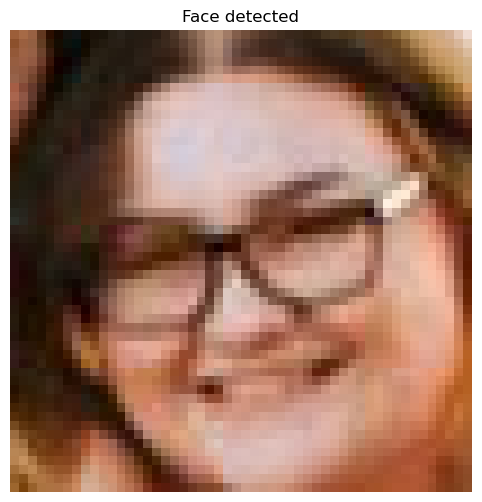

Segmentation and face detection

Previously, you learned how to make processes more computationally efficient with unsupervised superpixel segmentation. In this exercise, you’ll do just that!

Using the slic() function for segmentation, pre-process the image before passing it to the face detector.

Code

from skimage.segmentation import slic
from skimage.color import label2rgb

profile_image = imread('dataset/face_det9.jpg')

# Obtain the segmentation with default 100 regions
segments = slic(profile_image)

# Obtain segmented image using label2rgb
segmented_image = label2rgb(segments, profile_image, kind='avg')

# Detect the faces with multi scale method
detected = detector.detect_multi_scale(img=segmented_image, scale_factor=1.2,
                                       step_ratio=1,
                                       min_size=(10, 10),
                                       max_size=(1000, 1000))

# Show the detected faces
show_detected_face(segmented_image, detected)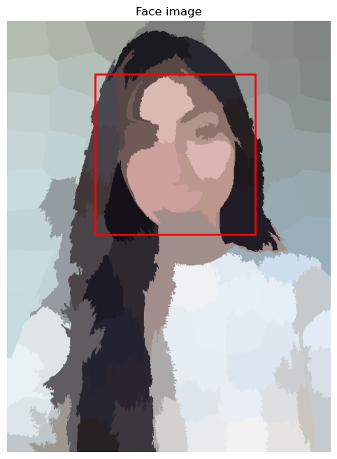

{'r': 108, 'c': 180, 'width': 328, 'height': 328}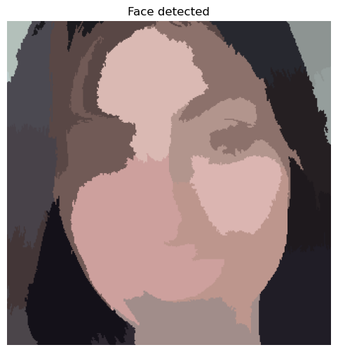

Real-world applications

Privacy protection

Let’s look at a real-world application of what you have learned in the course.

In this exercise, you will detect human faces in the image and for the sake of privacy, you will anonymize data by blurring people’s faces in the image automatically.

You can use the gaussian filter for the blurriness.

Code

def getFaceRectangle(image, d):
    ''' Extracts the face from the image using the coordinates of the detected image '''
    # X and Y starting points of the face rectangle
    x, y  = d['r'], d['c']

    # The width and height of the face rectangle
    width, height = d['r'] + d['width'],  d['c'] + d['height']

    # Extract the detected face
    face= image[ x:width, y:height]
    return face

def mergeBlurryFace(original, gaussian_image):
     # X and Y starting points of the face rectangle
    x, y  = d['r'], d['c']
    # The width and height of the face rectangle
    width, height = d['r'] + d['width'],  d['c'] + d['height']

    original[ x:width, y:height] = gaussian_image
    return original

Code

from skimage.filters import gaussian

group_image = imread('dataset/face_det25.jpg')
group_image_o = group_image.copy()

# Detect the faces
detected = detector.detect_multi_scale(img=group_image, scale_factor=1.2,
                                       step_ratio=1,
                                       min_size=(10, 10), max_size=(100, 100))

# For each detected face
for d in detected:
    # Obtain the face rectangle from detected coordinates
    face = getFaceRectangle(group_image, d)

    # Apply gaussian filter to extracted face
    blurred_face = gaussian(face, multichannel=True, sigma=8, preserve_range=True)

    # Merge this blurry face to our final image and show it
    resulting_image = mergeBlurryFace(group_image, blurred_face)

plot_comparison(group_image_o, resulting_image, 'Blurred faces')

/var/folders/gk/g6hht_993hbcv0ffg5wyh8f00000gn/T/ipykernel_5012/3288260764.py:17: FutureWarning: `multichannel` is a deprecated argument name for `gaussian`. It will be removed in version 1.0. Please use `channel_axis` instead.
  blurred_face = gaussian(face, multichannel=True, sigma=8, preserve_range=True)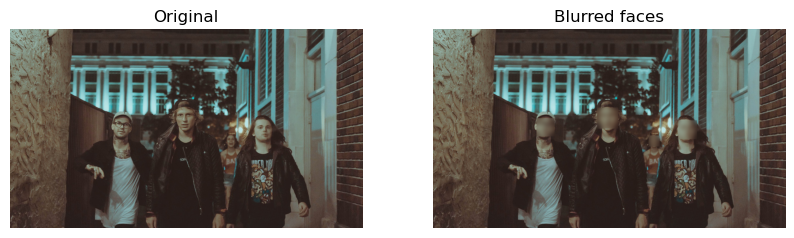

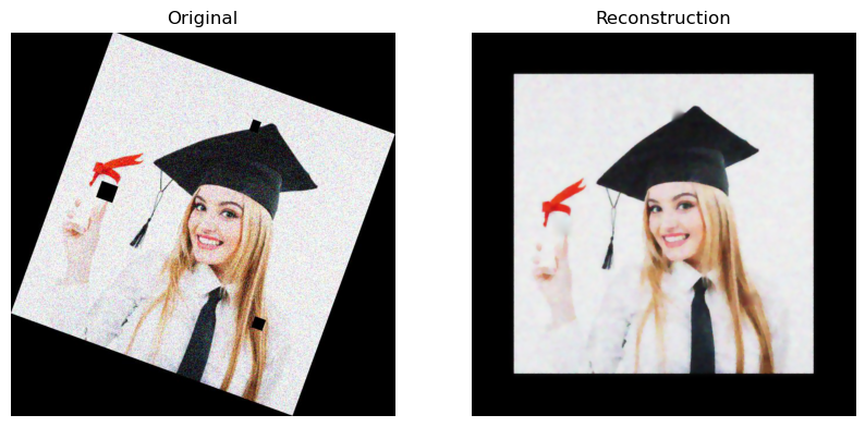
Help Sally restore her graduation photo

You are going to combine all the knowledge you acquired throughout the course to complete a final challenge: reconstructing a very damaged photo.

Help Sally restore her favorite portrait which was damaged by noise, distortion, and missing information due to a breach in her laptop.

You will be fixing the problems of this image by:

Rotating it to be uprightusing rotate()
Applying noise reduction with denoise_tv_chambolle()
Reconstructing the damaged parts with inpaint_biharmonic() from the inpaint module.

Code

def get_mask(image):
    # Create mask with three defect regions: left, middle, right respectively
    mask_for_solution = np.zeros(image.shape[:-1])
    mask_for_solution[450:475, 470:495] = 1
    mask_for_solution[320:355, 140:175] = 1
    mask_for_solution[130:155, 345:370] = 1
    return mask_for_solution

Code

from skimage.restoration import denoise_tv_chambolle, inpaint
from skimage import transform

damaged_image = imread('dataset/sally_damaged_image.jpg')

# Transform the image so it's not rotate
upright_img = transform.rotate(damaged_image, 20)

# Remove noise from the image, using the chambolle method
upright_img_without_noise = denoise_tv_chambolle(upright_img, weight=0.1, multichannel=True)

# Reconstruct the image missing parts
mask = get_mask(upright_img)
result = inpaint.inpaint_biharmonic(upright_img_without_noise, mask, multichannel=True)

# Show the resulting image
plot_comparison(damaged_image, result, "Reconstruction")

/var/folders/gk/g6hht_993hbcv0ffg5wyh8f00000gn/T/ipykernel_5012/3345107847.py:10: FutureWarning: `multichannel` is a deprecated argument name for `denoise_tv_chambolle`. It will be removed in version 1.0. Please use `channel_axis` instead.
  upright_img_without_noise = denoise_tv_chambolle(upright_img, weight=0.1, multichannel=True)
/var/folders/gk/g6hht_993hbcv0ffg5wyh8f00000gn/T/ipykernel_5012/3345107847.py:14: FutureWarning: `multichannel` is a deprecated argument name for `inpaint_biharmonic`. It will be removed in version 1.0. Please use `channel_axis` instead.
  result = inpaint.inpaint_biharmonic(upright_img_without_noise, mask, multichannel=True)